
1. CountVectorizer
CountVectorizer类会将文本中的词语转换为词频矩阵。 例如矩阵中包含一个元素a[i][j],它表示j词在i类文本下的词频。它通过fit_transform函数计算各个词语出现的次数,通过get_feature_names()可获取词袋中所有文本的关键字,通过toarray()可看到词频矩阵的结果。
from sklearn.feature_extraction.text import CountVectorizer
#语料
corpus = [
    'This is the first document.',
    'This is the this second second document.',
    'And the third one.',
    'Is this the first document?'
]
#将文本中的词转换成词频矩阵
vectorizer = CountVectorizer()
print(vectorizer)
#计算某个词出现的次数
X = vectorizer.fit_transform(corpus)
print(type(X),X)
#获取词袋中所有文本关键词
word = vectorizer.get_feature_names()
print(word)
#查看词频结果
print(X.toarray())
结果:
<class 'scipy.sparse._csr.csr_matrix'>   (np.int32(0), np.int32(8)) 1
  (np.int32(0), np.int32(3))    1
  (np.int32(0), np.int32(6))    1
  (np.int32(0), np.int32(2))    1
  (np.int32(0), np.int32(1))    1
  (np.int32(1), np.int32(8))    2
  (np.int32(1), np.int32(3))    1
  (np.int32(1), np.int32(6))    1
  (np.int32(1), np.int32(1))    1
  (np.int32(1), np.int32(5))    2
  (np.int32(2), np.int32(6))    1
  (np.int32(2), np.int32(0))    1
  (np.int32(2), np.int32(7))    1
  (np.int32(2), np.int32(4))    1
  (np.int32(3), np.int32(8))    1
  (np.int32(3), np.int32(3))    1
  (np.int32(3), np.int32(6))    1
  (np.int32(3), np.int32(2))    1
  (np.int32(3), np.int32(1))    1
['and', 'document', 'first', 'is', 'one', 'second', 'the', 'third', 'this']
[[0 1 1 1 0 0 1 0 1]
 [0 1 0 1 0 2 1 0 2]
 [1 0 0 0 1 0 1 1 0]
 [0 1 1 1 0 0 1 0 1]]
我们看下词的分布:
| and | document | first | is | one | second | the | third | this |
|---|---|---|---|---|---|---|---|---|
| 0 | 1 | 1 | 1 | 0 | 0 | 1 | 0 | 1 |
| 0 | 1 | 0 | 1 | 0 | 2 | 1 | 0 | 2 |
| 1 | 0 | 0 | 0 | 1 | 0 | 1 | 1 | 0 |
| 0 | 1 | 1 | 1 | 0 | 0 | 1 | 0 | 1 |
再看下原段落,可以验证以下分布是否正确(a[i][j],它表示j词在i类文本下的词频):
1:    'This is the first document.',
2:    'This is the this second second document.',
3:    'And the third one.',
4:    'Is this the first document?'
关于结果 X:
X = vectorizer.fit_transform(corpus):
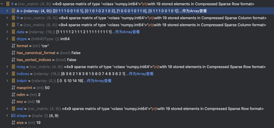
文档词频矩阵(稠密形式):
| 文档 | and | document | first | is | one | second | the | third | this | 非零值数量 |
|---|---|---|---|---|---|---|---|---|---|---|
| 1 | 0 | 1 | 1 | 1 | 0 | 0 | 1 | 0 | 1 | 5个 (1+1+1+1+1) |
| 2 | 0 | 1 | 0 | 1 | 0 | 2 | 1 | 0 | 2 | 6个 (1+1+2+1+2) |
| 3 | 1 | 0 | 0 | 0 | 1 | 0 | 1 | 1 | 0 | 4个 (1+1+1+1) |
| 4 | 0 | 1 | 1 | 1 | 0 | 0 | 1 | 0 | 1 | 4个 (1+1+1+1+1) |
| 总计 | - | - | - | - | - | - | - | - | - | 19个非零值 |
矩阵维度是4(文档数)×9(词汇量)=36,但实际非零元素只有19个(见X.data数组长度),因此X.size=19反映的是所有文档中实际出现的词汇计数总和
关于词汇表顺序:
vectorizer.get_feature_names() 返回的词汇列表按 字母升序 排列(从 a 到 z),这是 CountVectorizer 的默认行为。
在用户代码的语料中,词汇顺序为:
['and', 'document', 'first', 'is', 'one', 'second', 'the', 'third', 'this']
-
验证:
and(a开头)排最前,this(t开头)排最后。
📌 顺序调整方法
若需自定义顺序,可通过以下方式实现:
# 按词汇首次出现的顺序排序(非字母序)
vectorizer = CountVectorizer(vocabulary=sorted(set(" ".join(corpus).split())))
注意:默认字母序可确保结果可复现,不受语料输入顺序影响
2. TF-IDF
TF-IDF(term frequency-inverse document frequency)是文本加权方法,采用统计思想,即文本出现的次数和整个语料中文档频率来计算字词的重要度,是一种用于评估词在文档中重要性的统计方法,其核心思想是:词的重要性随其在文档中的出现频率正比增加,但随其在语料库中的普遍性反比下降。
什么是TF-IDF
TF-IDF是一种常用的文本处理技术,用以评估一个词对于一篇文章或语料库中一篇文章的重要性。TF代表词频(Term Frequency),IDF代表逆文档频率(Inverse Document Frequency)。字词的重要性随着它在文件中出现的次数成正比增加,但同时会随着它在语料库中出现的频率成反比下降。
TF-IDF的使用场景
TF-IDF常被用于文本分类、信息检索、关键词提取等领域。在文本分类中,可以根据TF-IDF值来计算文本与某个类别的相关程度;在信息检索中,可以根据用户输入的关键词的TF-IDF值来排序搜索结果;在关键词提取中,可以根据TF-IDF值来确定文本中的关键词。
TF-IDF原理
TF(全称TermFrequency)指的是某个词在文本中出现的频率。如果一个词在文本中出现的次数越多,那么它的TF值就越高。例如,在一篇文章中,词语“apple”出现了5次,而总词数为1000个,那么它的TF值为0.005。
这其中还有一个漏洞,就是 ”的“ ”是“ ”啊“ 等类似的词在文章中出现的此时是非常多的,但是这些大多都是没有意义词,对于判断文章的关键词几乎没有什么用处,我们称这些词为”停用词“,也就是说,在度量相关性的时候不应该考虑这些词的频率。
IDF(全称InverseDocumentFrequency)指的是一个词在文本集合中的重要程度。如果一个词在整个文本集合中出现的文档数越少,那么它的IDF值就越高,说明这个词在文本中的重要程度越高。例如,在一个由1000篇文章组成的文本集合中,词语“apple”只出现在10篇文章中,那么它的IDF值为log(1000/10) = 2。
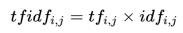
TF-IDF 值就是将TF和IDF相乘得到的结果。它反映了一个词在文本中的重要性。如果一个词在文本中出现的次数越多,同时在整个文本集合中出现的文档数越少,那么它的TF-IDF值就越高,说明这个词在文本中的重要程度越高。
TF-IDF的计算公式为:
优点:过滤一些常见但是无关紧要的字词。
TF(Term Frequency)表示某个关键词在整篇文章中出现的频率。(某个词在文章中出现的总次数/文章的总词数);
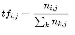
IDF(Inverse Document Frequency)表示计算倒文本频率。文本频率是指某个关键词在整个语料所有文章中出现的次数。倒文档频率又称为逆文档频率,它是文档频率的倒数,主要用于降低所有文档中一些常见却对文档影响不大的词语的作用。
默认:
这里, N为总的文档数,N(x)为包含这个词x的文档数。
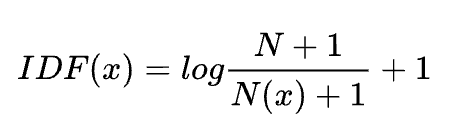
教科书标准的idf定义:
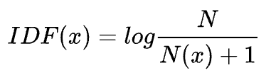
其中, N代表语料库的文档总数; N(x)代表包含该词x的文档数.
Tfidf 实现,一般是先通过countVectorizer, 然后再通过 tfidfTransformer, 转换成 tfidf 向量; 也有现成的 TfidfVectorizer API。
语句:
TfidfTransformer(norm='l2', use_idf=True, smooth_idf=True, sublinear_tf=False)示例:
from sklearn.feature_extraction.text import TfidfVectorizer, TfidfTransformer, CountVectorizer
import numpy as np
#语料
cc = [
      'aa bb.',
      'aa cc.'
]
# method 1
vectorizer = TfidfVectorizer()
X = vectorizer.fit_transform(cc)
print('feature',vectorizer.get_feature_names())
print(X.toarray())
结果:
feature ['aa', 'bb', 'cc']
[[0.57973867 0.81480247 0.        ]
[0.57973867 0. 0.81480247]]值得注意的是,默认语料会把单个字符当作停止单词(stop_words)进行过滤,如果需要保留单个字符组成的单词,可以修改分词方式:token_pattern='(?u)\\b\\w+\\b'
此外,上面还可实现如下:
# method 2
vectorizer=CountVectorizer()#token_pattern='(?u)\\b\\w+\\b'
transformer = TfidfTransformer()
cntTf = vectorizer.fit_transform(cc)
print('feature', vectorizer.get_feature_names())
print(cntTf)
cnt_array = cntTf.toarray()
X = transformer.fit_transform(cntTf)
print(X.toarray())
结果:
feature ['aa', 'bb', 'cc']
# 第一个数字表示第几个文档;第二个数字表示第几个feature,结果表示相应的词频。
  (0, 1)        1
  (0, 0)        1
  (1, 2)        1
  (1, 0)        1
[[0.57973867 0.81480247 0.        ]
[0.57973867 0. 0.81480247]]为了更加明白TfidfTransformer的操作,进行简单分解实现该功能:
# method 3
vectorizer=CountVectorizer()
cntTf = vectorizer.fit_transform(cc)
tf = cnt_array/np.sum(cnt_array, axis = 1, keepdims = True)
print('tf',tf)
idf = np.log((1+len(cnt_array))/(1+np.sum(cnt_array,axis = 0))) + 1
print('idf', idf)
t = tf*idf
print('tfidf',t)
print('norm tfidf', t/np.sqrt(np.sum(t**2, axis = 1, keepdims=True)))
结果:
tf [[0.5 0.5 0. ]
 [0.5 0.  0.5]]
idf [1.         1.40546511 1.40546511]
tfidf [[0.5        0.70273255 0.        ]
 [0.5        0.         0.70273255]]
norm tfidf [[0.57973867 0.81480247 0.        ]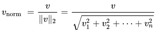
[0.57973867 0. 0.81480247]]也就是说,TfidfTransformer 默认会对获得的向量除以2范数进行归一化。
TF-IDF的信息论依据
一个查询(Query)中的每个关键词(Key Word)w的权重应该反映这个词查询来讲提供了多少信息。一个简单方法是用每个词的信息量作为他的权重。
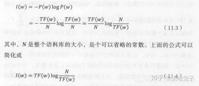
但是,如果两个词出现的频率 TF相同, 一个是某篇特定文章中的常见词,而另外一个词时分散在多篇文章中,显然第一个词有更高的分辨率,权重应该更大。
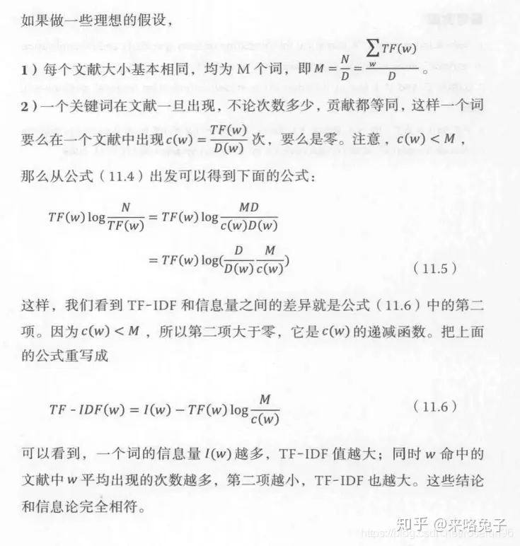
3. HashingVectorizer
语法
HashingVectorizer(alternate_sign=True, analyzer='word', binary=False,
         decode_error='strict', dtype=<class 'numpy.float64'>,
         encoding='utf-8', input='content', lowercase=True,
         n_features=1048576, ngram_range=(1, 1), non_negative=False,
         norm='l2', preprocessor=None, stop_words=None, strip_accents=None,
         token_pattern='(?u)\\b\\w\\w+\\b', tokenizer=None)
特点
普通的CountVectorizer存在但词库很大时,占用大内存,因此,使用hash技巧,并用稀疏矩阵存储编译后的矩阵,能很好解决这个问题。
实现的伪代码为:
 function hashing_vectorizer(features : array of string, N : integer):
     x := new vector[N]
     for f in features:
         h := hash(f)
         x[h mod N] += 1
return x这里伪代码没有考虑到hash冲突的情况,实际实现会更加复杂。
from sklearn.feature_extraction.text import HashingVectorizer
corpus = [
     'This is the first document.',
     'This document is the second document.',
     'And this is the third one.',
     'Is this the first document?',
 ]
vectorizer = HashingVectorizer(n_features=2**4)
X = vectorizer.fit_transform(corpus)
print(X.toarray())
print(X.shape)
结果:
[[-0.57735027  0.          0.          0.          0.          0.
   0.          0.         -0.57735027  0.          0.          0.
   0.          0.57735027  0.          0.        ]
 [-0.81649658  0.          0.          0.          0.          0.
   0.          0.          0.          0.          0.          0.40824829
   0.          0.40824829  0.          0.        ]
 [ 0.          0.          0.          0.         -0.70710678  0.70710678
   0.          0.          0.          0.          0.          0.
   0.          0.          0.          0.        ]
 [-0.57735027  0.          0.          0.          0.          0.
   0.          0.         -0.57735027  0.          0.          0.
   0.          0.57735027  0.          0.        ]]
(4, 16)
4. 总结
总的而言,这三种都是词袋模型的方法,其中,由于tfidfvectorizer这种方法可以降低高频信息量少词语的干扰,应用得更多。
reference: