一、VisionTransformer(VIT) 介绍
大模型已经成为人工智能领域的热门话题。在这股热潮中,大模型的核心结构 Transformer 也再次脱颖而出证明了其强大的能力和广泛的应用前景。 Transformer 自 2017年由 Google提出以来,便在 NLP领域掀起了一场革命。相较于传统的循环神经网络( RNN)和长短时记忆网络( LSTM), Transformer 凭借自注意力机制和端到端训练方式,以及处理长距离依赖问题上显著的优势,使其在多项 NLP任务中都取得了卓越表现,常见模型例如: BERT、 GPT 等。
随着 Transformer在 NLP领域的成功,慢慢的也开始进军到了 CV领域。在 CV 领域中,卷积神经网络( CNN)一直占据主导地位。然而, CNN 的卷积操作限制了其对全局信息的捕捉,导致在处理复杂场景时效果不佳。相比之下, Transformer 能够更好地捕捉长距离依赖关系,有助于识别图像中的全局特征,另外,自注意力机制也能使得模型关注到不同区域的重要信息,提高特征提取的准确性。
但是要想 Transformer 处理图像,首选需要考虑如何将图像转为序列数据,因为 CNN 的输入通常是一个四维张量,其维度通常表示为 [批次大小,高度,宽度,通道数],一般图像也是 RGB三维的,所以可以非常方便的处理图像数据。而 Transformer 的输入是一个三维张量,其维度表示为 [批次大小,序列长度,嵌入维度],维度的不同导致不能直接将图像传入 Transformer 结构 。
对此 VisionTransformer ( VIT)巧妙的例用了 CNN 解决了维度不一致的问题,成为了将 Transformer 架构应用于 CV 领域的一种创新方法, 下面是 VIT 的架构图:
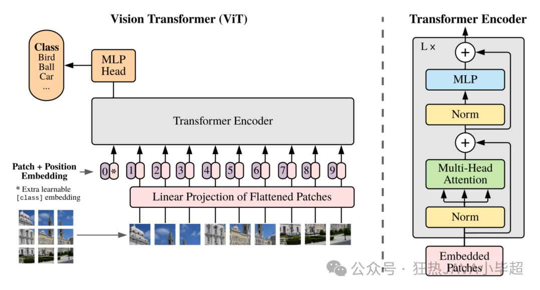
首先, VIT将输入图像分割成一系列固定大小的图像块(利用 CNN),每个块就像 NLP中的单词一样,成为序列中的一个元素,这点类似于文本模型中的 Embedding 层。这种分割方法使得图像的局部特征得以保留,并为后续的处理提供了基础。接着,为了确保模型能够理解图像块的空间位置,VIT为每个图像块添加了位置编码,这些编码是可学习的参数,它们准确地指示了每个块在原始图像中的位置。
然后,每个图像块被展平成一维向量,并通过一个线性层进行嵌入,转换成高维向量。这个过程类似于在自然语言处理中将单词映射到词嵌入向量。完成嵌入后,这些向量被送入标准的 Transformer编码器中。编码器由多个自注意力层和前馈网络组成,它们能够捕捉图像块之间的复杂交互和依赖关系。
最后, VIT在 Transformer编码器的输出上添加了一个分类头,通常是一个全连接层,用于生成最终的分类结果。
下面是 VIT-Base 的据图结构:
VisionTransformer(
  (conv_proj): Conv2d(3, 768, kernel_size=(16, 16), stride=(16, 16))
  (encoder): Encoder(
    (dropout): Dropout(p=0.0, inplace=False)
    (layers): Sequential(
      (encoder_layer_0): EncoderBlock(
        (ln_1): LayerNorm((768,), eps=1e-06, elementwise_affine=True)
        (self_attention): MultiheadAttention(
          (out_proj): NonDynamicallyQuantizableLinear(in_features=768, out_features=768, bias=True)
        )
        (dropout): Dropout(p=0.0, inplace=False)
        (ln_2): LayerNorm((768,), eps=1e-06, elementwise_affine=True)
        (mlp): MLPBlock(
          (0): Linear(in_features=768, out_features=3072, bias=True)
          (1): GELU(approximate='none')
          (2): Dropout(p=0.0, inplace=False)
          (3): Linear(in_features=3072, out_features=768, bias=True)
          (4): Dropout(p=0.0, inplace=False)
        )
      )
      (encoder_layer_1): EncoderBlock(
        (ln_1): LayerNorm((768,), eps=1e-06, elementwise_affine=True)
        (self_attention): MultiheadAttention(
          (out_proj): NonDynamicallyQuantizableLinear(in_features=768, out_features=768, bias=True)
        )
        (dropout): Dropout(p=0.0, inplace=False)
        (ln_2): LayerNorm((768,), eps=1e-06, elementwise_affine=True)
        (mlp): MLPBlock(
          (0): Linear(in_features=768, out_features=3072, bias=True)
          (1): GELU(approximate='none')
          (2): Dropout(p=0.0, inplace=False)
          (3): Linear(in_features=3072, out_features=768, bias=True)
          (4): Dropout(p=0.0, inplace=False)
        )
      )
      ...
      (encoder_layer_11): EncoderBlock(
        (ln_1): LayerNorm((768,), eps=1e-06, elementwise_affine=True)
        (self_attention): MultiheadAttention(
          (out_proj): NonDynamicallyQuantizableLinear(in_features=768, out_features=768, bias=True)
        )
        (dropout): Dropout(p=0.0, inplace=False)
        (ln_2): LayerNorm((768,), eps=1e-06, elementwise_affine=True)
        (mlp): MLPBlock(
          (0): Linear(in_features=768, out_features=3072, bias=True)
          (1): GELU(approximate='none')
          (2): Dropout(p=0.0, inplace=False)
          (3): Linear(in_features=3072, out_features=768, bias=True)
          (4): Dropout(p=0.0, inplace=False)
        )
      )
    )
    (ln): LayerNorm((768,), eps=1e-06, elementwise_affine=True)
  )
  (heads): Sequential(
    (head): Linear(in_features=768, out_features=1000, bias=True)
  )
)
从结构中可以看出,输入三维图像, 经过 (16,16) 的卷积核,并且步长也是 (16,16) ,如果输入大小为 (224,224) ,则输出就为 768 个大小为 (14,14) 的特征图,然后每个特征图在展平成一维向量就是 (batch,768,196) ,接着后面就可以喂入到 Transformer 结构了。
上面对 VIT 有了简单的了解后,下卖弄使用 Pytorch vit_b_16 模型 FineTune 训练下 Kaggle 比赛中的驾驶员状态数据集。
实验使用的依赖版本如下:
torch==1.13.1+cu116
torchvision==0.14.1+cu116
tensorboard==2.17.1
tensorboard-data-server==0.7.2
二、准备数据集
驾驶员状态数据集这里使用 Kaggle 比赛的数据,由于官网已经没办法下载了,这里可以在 百度的 aistudio 公开数据集中下载:
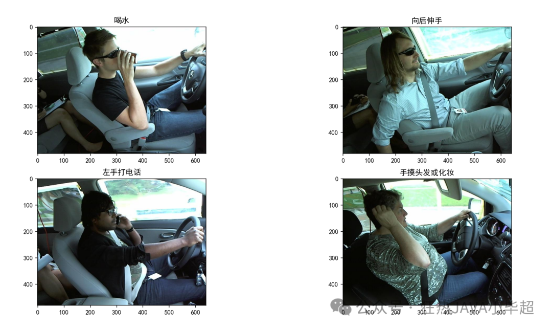
下载后可以看到训练集下有 10个分类:
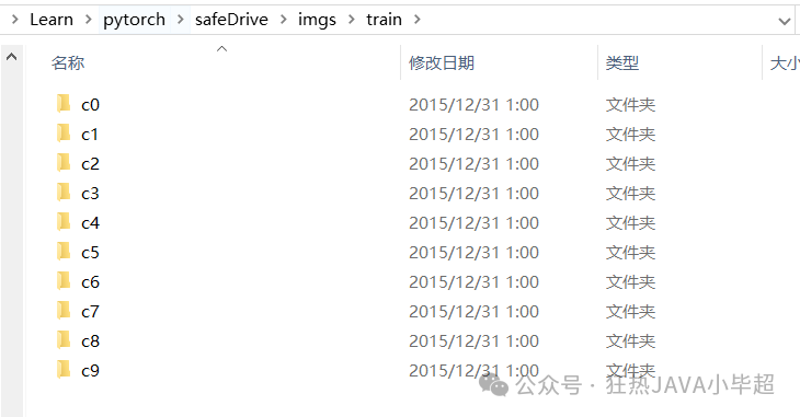 分别表示:
分别表示:
| 分类 | 解释 |
|---|---|
| c0 | 安全驾驶 |
| c1 | 右手使用手机 |
| c2 | 右手打电话 |
| c3 | 左手使用手机 |
| c4 | 左手打电话 |
| c5 | 操作中控台 |
| c6 | 喝水 |
| c7 | 向后伸手 |
| c8 | 手摸头发或化妆 |
| c9 | 与人交谈 |
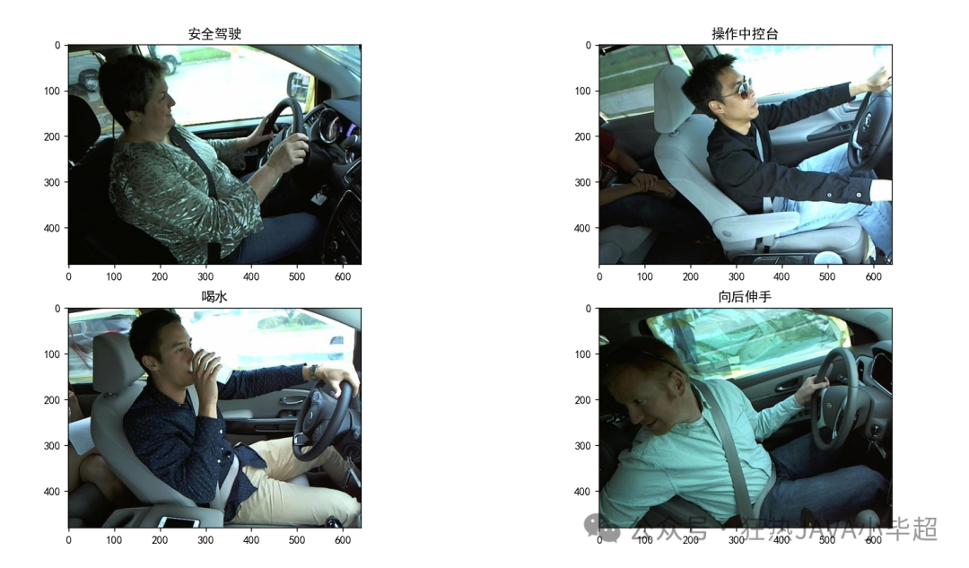
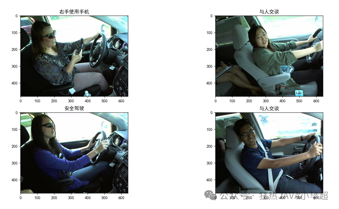
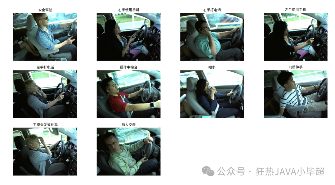
每个类别下的示例图像如下:
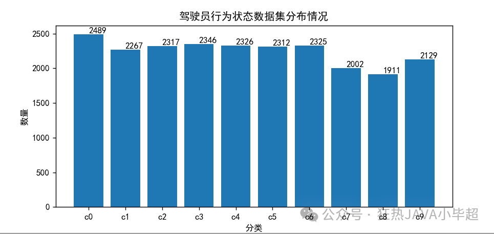
数据集的分布如下,每个类别整体分布 2000 左右:
三、VIT FineTune 训练
在 Pytorch 中已经集成好了 VIT 结构,这里使用 vit_b_16 为例,可以选择冻结所有原来模型的参数,追加两层全链接层:
net.py
import torch.nn as nn
from torchvision import models

class Model(nn.Module):
    def __init__(self, num_classes):
        super(Model, self).__init__()

        # 加载预训练的 vit_b_16 模型
        self.base_model = models.vit_b_16(pretrained=True)
        print(self.base_model)

        # 冻结主干网络的权重
        for param in self.base_model.parameters():
            param.requires_grad = False

        # 自定义分类头
        self.relu = nn.ReLU()
        self.fc1 = nn.Linear(self.base_model.heads.head.out_features, 1024)
        self.dropout1 = nn.Dropout(p=0.2)
        self.fc2 = nn.Linear(1024, 512)
        self.dropout2 = nn.Dropout(p=0.1)
        self.fc3 = nn.Linear(512, num_classes)

    def forward(self, x):
        x = self.base_model(x)
        x = self.fc1(x)
        x = self.relu(x)
        x = self.dropout1(x)
        x = self.fc2(x)
        x = self.relu(x)
        x = self.dropout2(x)
        x = self.fc3(x)
        return x
或者不冻结原有的参数,也不改变原来模型的结构,在此基础上继续训练新的类别,可以使用如下结构,直接将 head 层的输出改为分类的大小:
net.py
import torch.nn as nn
from torchvision import models

class Model(nn.Module):
    def __init__(self, num_classes):
        super(Model, self).__init__()

        # 加载预训练模型
        self.base_model = models.vit_b_16(pretrained=True)
        print(self.base_model)

        # 获取输入特征维度
        num_ftrs = self.base_model.heads.head.in_features

        # 修改最后一层的输出数
        self.base_model.heads.head = nn.Linear(num_ftrs, num_classes)
        print(self.base_model)

    def forward(self, x):
        return self.base_model(x)
这里我使用第一种方式,显存占用比较小,整体训练过程如下,其中使用 80% 的数据训练,20% 的数据验证:
import os
import json
import sys
import torch
import torch.nn as nn
import torch.optim as optim
from torch.utils.data import DataLoader, random_split
from torch.utils.tensorboard import SummaryWriter
from torchvision import datasets, models, transforms
from tqdm import tqdm
from net import Model
# 设置随机种子,让结果可复现
torch.manual_seed(0)
def load_data(data_dir, train_ratio, data_transforms, batch_size):
"""加载数据集并分割为训练集和验证集"""
# 读取数据集
dataset = datasets.ImageFolder(data_dir, data_transforms)
# 拆分为训练集和验证集
train_size = int(train_ratio * len(dataset))
val_size = len(dataset) - train_size
train_dataset, val_dataset = random_split(dataset, [train_size, val_size])
train_loader = DataLoader(train_dataset, batch_size=batch_size, shuffle=True)
val_loader = DataLoader(val_dataset, batch_size=batch_size, shuffle=False)
return train_loader, val_loader, dataset.classes
def validate_model(model, val_loader, device, criterion):
"""验证模型性能"""
model.eval()
correct = 0
total = 0
running_loss = 0.0
with torch.no_grad():
for inputs, labels in tqdm(val_loader, file=sys.stdout, desc="Validation"):
inputs, labels = inputs.to(device), labels.to(device)
outputs = model(inputs)
loss = criterion(outputs, labels)
running_loss += loss.item()
_, predicted = torch.max(outputs, 1)
total += labels.size(0)
correct += (predicted == labels).sum().item()
accuracy = 100 * correct / total
avg_loss = running_loss / len(val_loader)
return accuracy, avg_loss
def train_model(model, criterion, optimizer, train_loader, val_loader, device, output_dir, writer, num_epochs=10):
"""训练模型"""
best_accuracy = 0.0
global_step = 0
for epoch in range(num_epochs):
# 训练阶段
model.train()
running_loss = 0.0
for inputs, labels in tqdm(train_loader, file=sys.stdout, desc=f"Train Epoch {epoch+1}/{num_epochs}"):
inputs, labels = inputs.to(device), labels.to(device)
optimizer.zero_grad()
outputs = model(inputs)
loss = criterion(outputs, labels)
loss.backward()
optimizer.step()
running_loss += loss.item()
writer.add_scalar('Loss/train', loss.item(), global_step)
global_step += 1
train_loss = running_loss / len(train_loader)
# 验证阶段
accuracy, val_loss = validate_model(model, val_loader, device, criterion)
# 记录日志
tqdm.write(f'Epoch {epoch+1}/{num_epochs}, Device: {device}')
tqdm.write(f'Train Loss: {train_loss:.4f}, Val Loss: {val_loss:.4f}, Accuracy: {accuracy:.2f}%')
writer.add_scalar('Loss/val', val_loss, epoch)
writer.add_scalar('Accuracy/val', accuracy, epoch)
# 保存最佳模型
if accuracy > best_accuracy:
torch.save(model.state_dict(), os.path.join(output_dir, 'best_model.pth'))
best_accuracy = accuracy
tqdm.write(f'New best model saved with accuracy: {accuracy:.2f}%')
# 保存最终模型
torch.save(model.state_dict(), os.path.join(output_dir, 'last_model.pth'))
tqdm.write(f'Training completed. Best accuracy: {best_accuracy:.2f}%')
def main():
"""主函数"""
# 配置参数
data_dir = 'imgs/train'
output_dir = "model"
logs_dir = "logs"
train_ratio = 0.8
batch_size = 45
learning_rate = 1e-3
num_epochs = 50
# 数据预处理
data_transforms = transforms.Compose([
transforms.Resize(256),
transforms.CenterCrop(224),
transforms.ToTensor(),
transforms.Normalize([0.485, 0.456, 0.406], [0.229, 0.224, 0.225])
])
# 创建输出目录
if not os.path.exists(output_dir):
os.makedirs(output_dir)
# 加载数据集
train_loader, val_loader, classes = load_data(
data_dir=data_dir,
train_ratio=train_ratio,
data_transforms=data_transforms,
batch_size=batch_size
)
# 保存类别信息
with open(os.path.join(output_dir, "classify.txt"), "w", encoding="utf-8") as f:
json.dump(classes, f, ensure_ascii=False, indent=2)
print(f"Dataset loaded: {len(classes)} classes")
print(f"Classes: {classes}")
# 设置设备
device = torch.device("cuda:0" if torch.cuda.is_available() else "cpu")
print(f"Using device: {device}")
# 初始化模型
model = Model(len(classes))
print("Model architecture:")
print(model)
# 损失函数和优化器
criterion = nn.CrossEntropyLoss()
optimizer = optim.AdamW(model.parameters(), lr=learning_rate)
# TensorBoard记录器
writer = SummaryWriter(logs_dir)
# 训练模型
model.to(device)
train_model(
model=model,
criterion=criterion,
optimizer=optimizer,
train_loader=train_loader,
val_loader=val_loader,
device=device,
output_dir=output_dir,
writer=writer,
num_epochs=num_epochs
)
writer.close()
print("Training completed!")
if __name__ == '__main__':
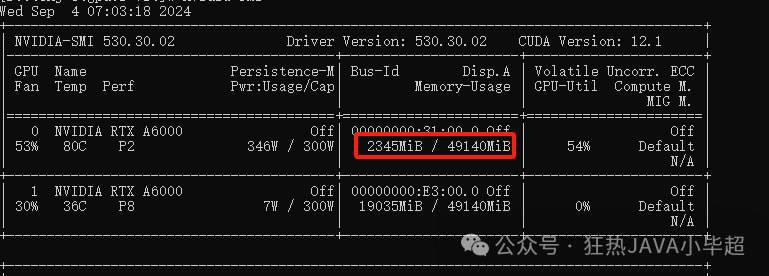
main()训练期间大概占用显存两个 G左右:
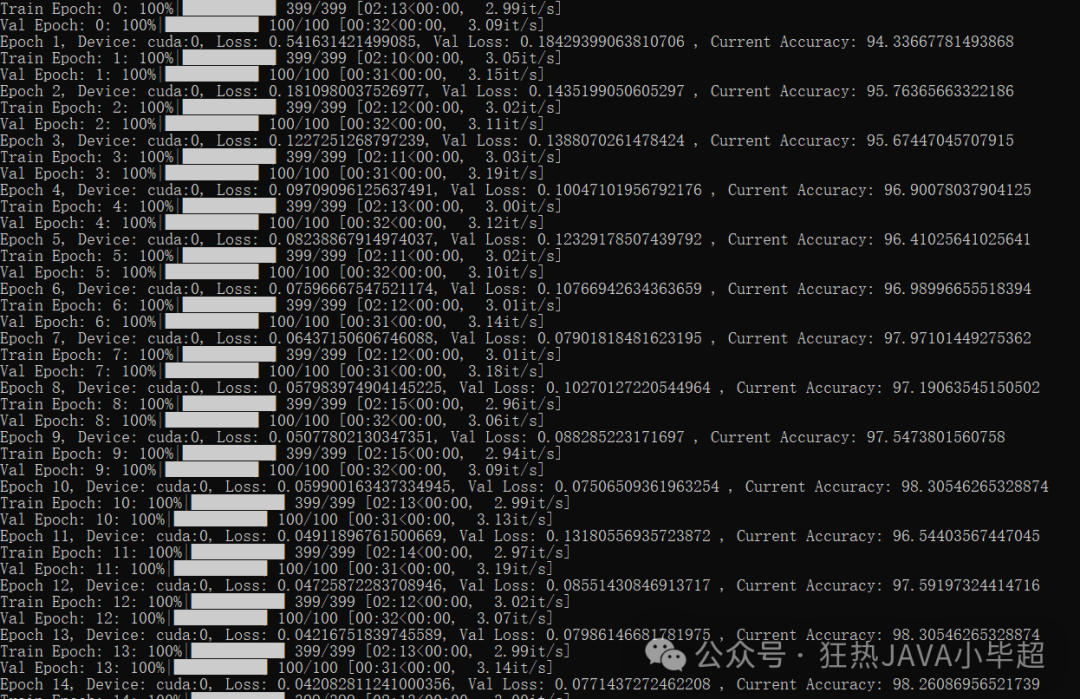
训练过程,可以看到验证集的准确率在逐步提升以及 loss在逐步收敛:
训练结束后,可以查看下 tensorboard 中你的 loss 和 准确率的曲线:
tensorboard --logdir=logs --bind_all在 浏览器访问 http:ip:6006/
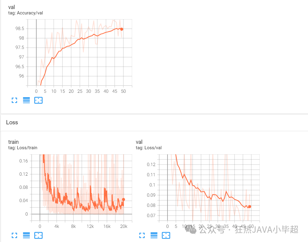
在验证集上的准确率达到 98.5 左右, loss 的波动还是蛮大的,大家也可以加入更多优化策略进来。
四、模型测试
import os
import json
import torch
import matplotlib.pyplot as plt
from PIL import Image
from torchvision import transforms
from net import Model

# 设置中文字体
plt.rcParams['font.sans-serif'] = ['SimHei']
plt.rcParams['axes.unicode_minus'] = False  # 解决负号显示问题

# 分类标签中文映射
classify_cn = {
    "c0": "安全驾驶",
    "c1": "右手使用手机",
    "c2": "右手打电话",
    "c3": "左手使用手机",
    "c4": "左手打电话",
    "c5": "操作中控台",
    "c6": "喝水",
    "c7": "向后伸手",
    "c8": "手摸头发或化妆",
    "c9": "与人交谈"
}

def predict_image(model, image_path, data_transforms, device, classify, classify_cn):
    """预测单张图像的类别"""
    # 加载和预处理图像
    image = Image.open(image_path).convert('RGB')
    input_tensor = data_transforms(image).unsqueeze(0).to(device)

    # 模型预测
    model.eval()
    with torch.no_grad():
        output = model(input_tensor)
        _, predicted = torch.max(output.data, 1)
        predicted_idx = predicted[0].item()

    # 获取预测标签
    class_id = classify[predicted_idx]
    label = classify_cn.get(class_id, f"未知类别({class_id})")
    confidence = torch.softmax(output, 1)[0][predicted_idx].item()

    return image, label, confidence

def main():
    # 配置参数
    image_dir = "imgs/test"
    model_path = "model/best_model.pth"
    classify_file = "model/classify.txt"

    # 读取分类标签
    try:
        with open(classify_file, "r", encoding="utf-8") as f:
            classify = json.load(f)
        print(f"加载分类标签成功,共{len(classify)}个类别")
    except FileNotFoundError:
        print(f"错误:找不到分类文件 {classify_file}")
        return
    except json.JSONDecodeError:
        print("错误:分类文件格式不正确")
        return

    # 设置设备
    device = torch.device("cuda:0" if torch.cuda.is_available() else "cpu")
    print(f"使用设备: {device}")

    # 加载模型
    try:
        model = Model(len(classify))
        model.load_state_dict(torch.load(model_path, map_location=device))
        model = model.to(device)
        print("模型加载成功")
    except FileNotFoundError:
        print(f"错误:找不到模型文件 {model_path}")
        return
    except Exception as e:
        print(f"模型加载失败: {e}")
        return

    # 数据预处理
    data_transforms = transforms.Compose([
        transforms.Resize(224),
        transforms.CenterCrop(224),
        transforms.ToTensor(),
        transforms.Normalize([0.485, 0.456, 0.406], [0.229, 0.224, 0.225])
    ])

    # 获取测试图像
    try:
        image_files = [f for f in os.listdir(image_dir)
                      if f.lower().endswith(('.png', '.jpg', '.jpeg'))]
        if not image_files:
            print(f"在目录 {image_dir} 中未找到图像文件")
            return
        print(f"找到 {len(image_files)} 张测试图像")
    except FileNotFoundError:
        print(f"错误:找不到测试目录 {image_dir}")
        return

    # 将图像分成4个一组进行显示
    image_groups = [image_files[i:i+4] for i in range(0, len(image_files), 4)]

    for group_idx, image_names in enumerate(image_groups):
        # 创建子图
        fig, axes = plt.subplots(2, 2, figsize=(12, 10))
        fig.suptitle(f'图像分类预测结果 (第{group_idx + 1}组)', fontsize=16, fontweight='bold')

        for i, image_name in enumerate(image_names):
            row, col = i // 2, i % 2
            ax = axes[row, col]

            try:
                image_path = os.path.join(image_dir, image_name)
                image, label, confidence = predict_image(
                    model, image_path, data_transforms, device, classify, classify_cn
                )

                # 显示图像和预测结果
                ax.imshow(image)
                ax.set_title(f'{label}\n置信度: {confidence:.2%}', fontsize=12)
                ax.axis('off')

                # 在图像文件名下方显示文件名
                ax.text(0.5, -0.1, image_name, transform=ax.transAxes,
                       ha='center', fontsize=9, style='italic')

            except Exception as e:
                print(f"处理图像 {image_name} 时出错: {e}")
                ax.text(0.5, 0.5, f"加载失败\n{image_name}",
                       ha='center', va='center', transform=ax.transAxes)
                ax.axis('off')

        # 隐藏多余的子图
        for i in range(len(image_names), 4):
            row, col = i // 2, i % 2
            axes[row, col].axis('off')

        plt.tight_layout()
        plt.subplots_adjust(top=0.92)
        plt.show()

        # 询问是否继续显示下一组
        if group_idx < len(image_groups) - 1:
            continue_input = input("按Enter继续显示下一组,输入q退出: ")
            if continue_input.lower() == 'q':
                break

if __name__ == '__main__':
    main()