02-pytorch基础语法

常用模块以及设置

import torch
import numpy as np
from matplotlib import pyplot as plt

dtype = torch.double
# GPU运算
device = torch.device("cuda")
# GPU运算方案推荐写法：
device = torch.device('cuda:0' if torch.cuda.is_available() else 'cpu')
****.to(device, 可以转换类型)
# “:0 表示在哪个显卡上进行运算，单显卡不写与写上:0可以划等号，不写自动分配”

# 推进GPU运算：
import torch

dtype = torch.double
# GPU运算
device = torch.device("cuda")
device = torch.device('cuda:0' if torch.cuda.is_available() else 'cpu')

a = torch.rand(3, 4, device=device)
b = torch.rand(4)

c1 = a - b
c2 = torch.sub(a, b)
c2.to(device)
print(c2)

张量

官方文档：torch.Tensor — PyTorch 2.1 documentation

什么是张量

在深度学习里，张量可以将向量和矩阵推广到任意维度，其实就是多维数组。

张量的维度（rank，number of dimensions）指的是张量中用来索引元素的索引个数，0维张量就是标量，因为不需要索引，而对于向量（vector）而言，只需要一个索引就可以得到相应元素，后续同理。高维的张量其实就是对低维张量的堆叠。

张量的形状（shape，number of rows and columns）指的是张量中每一维度的大小。

张量的类型（type，data type of tensor's elements）指的是张量中每个元素的数据类型。

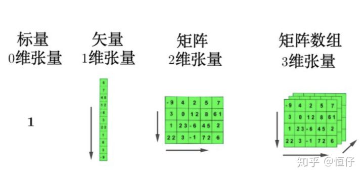
现在将三维的张量用一个正方体来表示：

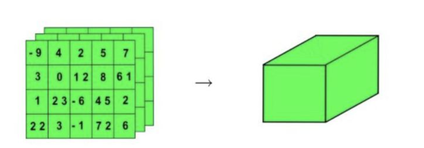
这样子可以进一步生成更高维的张量：

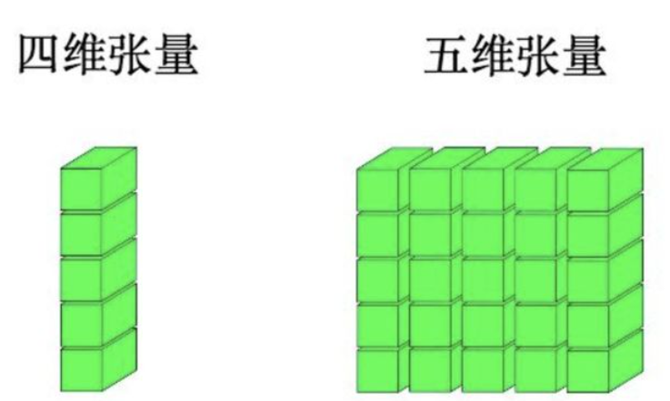
这有啥用呢？在用TensorFlow处理更高维数据结构的时候，最好可以能够在脑子里相出数据的形状。

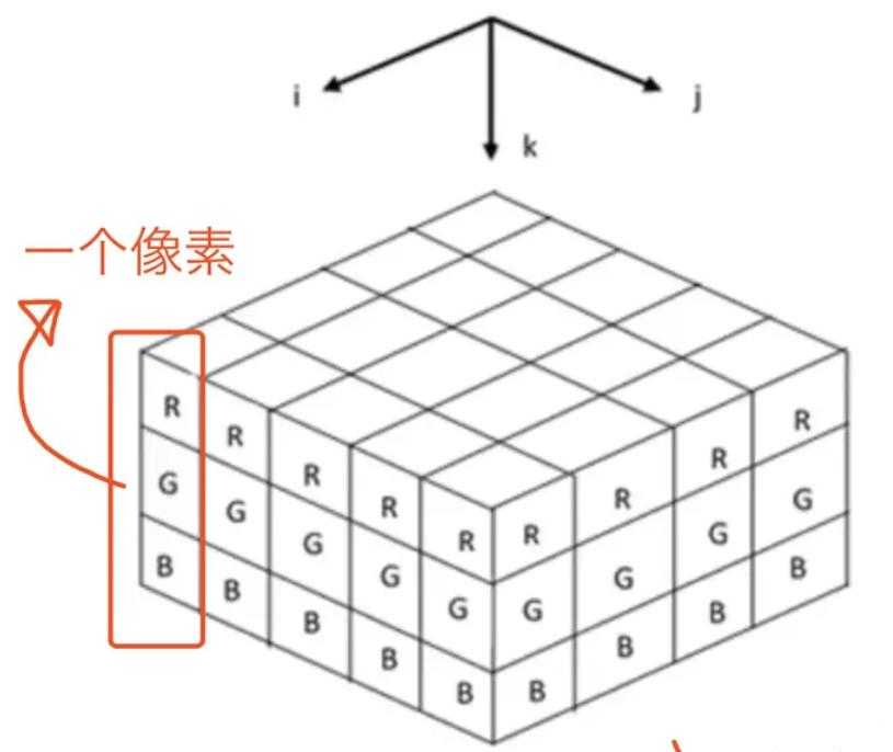
举个简单的例子，彩色图像文件（RGB）一般都会处理成3-d tensor，每个2d array中的element表示一个像素，R代表Red，G代表Green，B代表Blue：

而用Python举例子的话，来看看下面这个表格：

阶	数学实例	Python例子
0	纯量（只有大小）	s = 483
1	向量（大小和方向）	v = [1.1, 2.2, 3.3]
2	矩阵（数据表）	m = [[1,2,3], [4,5,6], [7,8,9]]
3	3阶张量（数据立体）	t = [[[2], [4], [6]], [[8], [10], [12]], [[14], [16], [18]]]
n	n阶（自己想想看）	... ...

数据类型dtype

张量构造函数（例如tensor()，zeros()...）在执行的时候，其实有个参数是叫dtype的

a = torch.ones(3,224,224, dtype=torch.int32)

dtype制定了张量中每个元素的类型。在PyTorch中有一些基本的数据类型，和NumPy类型故意设计的相似：

类型	说明
torch.float32/torch.float	32位浮点数-默认
torch.float64/torch.double	64位双精度浮点数
torch.float16/torch.half	16位半精度浮点数
torch.int8	8位有符号整数
torch.uint8	8位无符号整数
torch.int16或torch.short	16位有符号整数
torch.int32或http://torch.int	32位有符号整数
torch.int64或torch.long	64位有符号整数
torch.bool	布尔型

打开源代码查看更多类型,至于有什么屌用，我也不到，碰到再说：

float32: dtype = ...
float: dtype = ...
float64: dtype = ...
double: dtype = ...
float16: dtype = ...
bfloat16: dtype = ...
half: dtype = ...
uint8: dtype = ...
int8: dtype = ...
int16: dtype = ...
short: dtype = ...
int32: dtype = ...
int: dtype = ...
int64: dtype = ...
long: dtype = ...
complex32: dtype = ...
complex64: dtype = ...
cfloat: dtype = ...
complex128: dtype = ...
cdouble: dtype = ...
quint8: dtype = ...
qint8: dtype = ...
qint32: dtype = ...
bool: dtype = ...
quint4x2: dtype = ...
quint2x4: dtype = ...

要注意，采用更高的精度如64位，并不会提高模型精度，相反需要更多的内存和计算时间。16位半精度浮点数的数据类型在标准CPU中并不存在，而是由现代GPU提供。如果需要的话，可以切换到这种方式来减少神经网络的占用空间，这样对精度损失也会比较小。

那么，如何改变张量a的类型呢？可以通过to()方法：

a = a.to(torch.float)
a.dtype  # torch.float32

创建张量

import torch
import numpy as np
from matplotlib import pyplot as plt
dtype = torch.double
device = torch.device("cuda:0")

# 转化np矩阵
>>>li = [[402, 754, 327, 979], [713, 926, 879, 934], [540, 953, 209, 369]]
>>>torch.Tensor(li)
>>>tensor([[402., 754., 327., 979.],
        [713., 926., 879., 934.],
        [540., 953., 209., 369.]])

# 创建一维等距向量
>>>torch.linspace(0, 1, 100, dtype=torch.double, 
                  # device=device
                  )
>>>tensor([0.0000, 0.0101, 0.0202, 0.0303, 0.0404, 0.0505, 0.0606, 0.0707, 0.0808,
        0.0909, 0.1010, 0.1111, 0.1212, 0.1313, 0.1414, 0.1515, 0.1616, 0.1717,
        0.1818, 0.1919, 0.2020, 0.2121, 0.2222, 0.2323, 0.2424, 0.2525, 0.2626,
        0.2727, 0.2828, 0.2929, 0.3030, 0.3131, 0.3232, 0.3333, 0.3434, 0.3535,
        0.3636, 0.3737, 0.3838, 0.3939, 0.4040, 0.4141, 0.4242, 0.4343, 0.4444,
        0.4545, 0.4646, 0.4747, 0.4848, 0.4949, 0.5051, 0.5152, 0.5253, 0.5354,
        0.5455, 0.5556, 0.5657, 0.5758, 0.5859, 0.5960, 0.6061, 0.6162, 0.6263,
        0.6364, 0.6465, 0.6566, 0.6667, 0.6768, 0.6869, 0.6970, 0.7071, 0.7172,
        0.7273, 0.7374, 0.7475, 0.7576, 0.7677, 0.7778, 0.7879, 0.7980, 0.8081,
        0.8182, 0.8283, 0.8384, 0.8485, 0.8586, 0.8687, 0.8788, 0.8889, 0.8990,
        0.9091, 0.9192, 0.9293, 0.9394, 0.9495, 0.9596, 0.9697, 0.9798, 0.9899,
        1.0000], dtype=torch.float64)

# 创建全一矩阵，零矩阵
>>>torch.ones(3, 4, dtype=dtype)
>>>tensor([[1., 1., 1., 1.],
        [1., 1., 1., 1.],
        [1., 1., 1., 1.]], dtype=torch.float64)
>>>torch.zeros(3,4,dtype=dtype)
>>>tensor([[0., 0., 0., 0.],
        [0., 0., 0., 0.],
        [0., 0., 0., 0.]], dtype=torch.float64)

# 创建随机矩阵
x = torch.rand(n, m, dtype=dtype, device=device)
x = torch.randn(n, m, dtype=dtype, device=device)
x = torch.normal(means, std, dtype=dtype, device=device)

新建Tensor的几种方法

函数	功能
Tensor(*sizes)	基础构造函数
tensor(data,)	类似np.array的构造函数
ones(*sizes)	全1Tensor
zeros(*sizes)	全0Tensor
eye(*sizes)	对角线为1，其他为0
arange(s,e,step)	从s到e，步长为step
linspace(s,e,steps)	从s到e，均匀切分成steps份
rand/randn(*sizes)	均匀/标准正态分布
normal(mean,std)/uniform(from,to)	正态分布/均匀分布
randperm(m)	随机排列

张量操作

# 增加维度
x = x.unsqueeze(dim)    # dim=0,1,...

# 转置
x = x.t()

# 大小
print(x.size())

# 切片
x_1 = x[:,1:-2]

常用函数

# 数学函数
y = torch.sin(x)
y = torch.tan(x)
y = torch.atan(x)
y = torch.sqrt(x)
y = torch.relu(x)
y = torch.tanh(x)
y = torch.sigmoid(x)

# 其他函数
y = torch.sum(x, dim = 0)

Tensor/张量的基本运算

1. 加法运算

import torch

# 这两个Tensor加减乘除会对b自动进行Broadcasting
a = torch.rand(3, 4)
b = torch.rand(4)

c1 = a + b
c2 = torch.add(a, b)
print(c1.shape, c2.shape)
print(torch.all(torch.eq(c1, c2)))

打印结果：

torch.Size([3, 4]) torch.Size([3, 4])
tensor(True)

2. 减法运算

a = torch.rand(3, 4)
b = torch.rand(4)

c1 = a - b
# 使用PyTorch的sub函数来执行元素级的减法
c2 = torch.sub(a, b)
print(c1.shape, c2.shape)
print(torch.all(torch.eq(c1, c2)))

打印结果：

torch.Size([3, 4]) torch.Size([3, 4])
tensor(1, dtype=torch.uint8)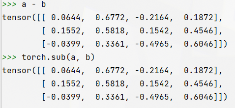

3. 哈达玛积(element wise，对应元素相乘)

c1 = a * b
c2 = torch.mul(a, b)
print(c1.shape, c2.shape)
print(torch.all(torch.eq(c1, c2)))

打印结果：

torch.Size([3, 4]) torch.Size([3, 4])
tensor(1, dtype=torch.uint8)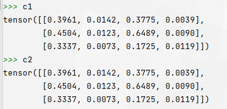

4. 除法运算

c1 = a / b
c2 = torch.div(a, b)
print(c1.shape, c2.shape)
print(torch.all(torch.eq(c1, c2)))

打印结果：

torch.Size([3, 4]) torch.Size([3, 4])
tensor(1, dtype=torch.uint8)

5. 矩阵乘法

5.1 二维矩阵相乘

二维矩阵乘法运算操作包括

• torch.mm()：只适用于2维数据
• torch.matmul()：适用于所有维度数据
• @：适用于所有维度数据

import torch

a = torch.ones(2, 1)
b = torch.ones(1, 2)
print(torch.mm(a, b).shape)
print(torch.matmul(a, b).shape)
print((a @ b).shape)

打印结果：

torch.Size([2, 2])
torch.Size([2, 2])
torch.Size([2, 2])

5.2 多维矩阵相乘

对于高维的Tensor（dim>2），定义其矩阵乘法仅在最后的两个维度上，要求前面的维度必须保持一致，就像矩阵的索引一样并且运算操只有torch.matmul()。

c = torch.rand(4, 3, 28, 64)
d = torch.rand(4, 3, 64, 32)
print(torch.matmul(c, d).shape)

打印结果：

torch.Size([4, 3, 28, 32])

注意，在这种情形下的矩阵相乘，前面的"矩阵索引维度"如果符合Broadcasting机制，也会自动做广播，然后相乘。示例代码：

c = torch.rand(4, 3, 28, 64)
d = torch.rand(4, 1, 64, 32)
print(torch.matmul(c, d).shape)

打印结果：

torch.Size([4, 3, 28, 32])

6. 幂运算

import torch

a = torch.full([2, 2], 3)
b = a.pow(2) # 也可以a**2
print(b)

打印结果：

tensor([[9, 9],
        [9, 9]])

7. 开方运算

c = b.sqrt() # 也可以a**(0.5)
print(c)
d = b.rsqrt() # 平方根的倒数
print(d)

打印结果：

tensor([[3., 3.],
        [3., 3.]])
tensor([[0.3333, 0.3333],
        [0.3333, 0.3333]])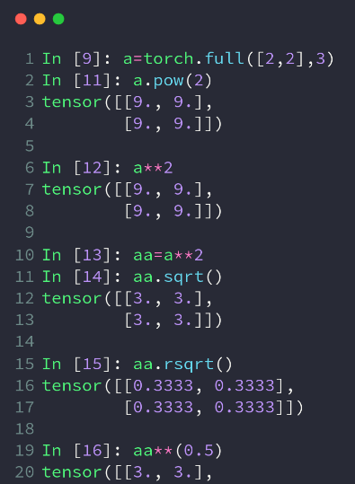

8.指数与对数运算

注意log是以自然对数为底数的，以2为底的用log2，以10为底的用log10

import torch

a = torch.exp(torch.ones(2, 2)) # 得到2*2的全是e的Tensor
print(a)
print(torch.log(a)) # 取自然对数

打印结果：

tensor([[2.7183, 2.7183],
        [2.7183, 2.7183]])
tensor([[1.0000, 1.0000],
        [1.0000, 1.0000]])

9.近似值运算

import torch

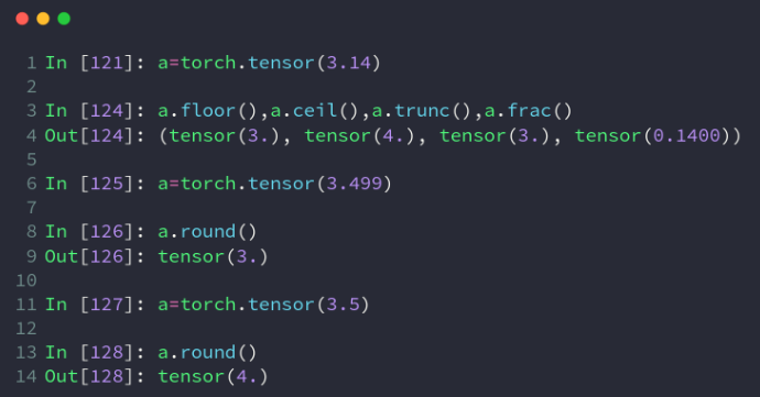
a = torch.tensor(3.14)
print(a.floor(), a.ceil(), a.trunc(), a.frac()) # 取下,取上,取整数,取小数
b = torch.tensor(3.49)
c = torch.tensor(3.5)
print(b.round(), c.round()) # 四舍五入

打印结果：

tensor(3.) tensor(4.) tensor(3.) tensor(0.1400)
tensor(3.) tensor(4.)

10. 裁剪运算

即对Tensor中的元素进行范围过滤，不符合条件的可以把它变换到范围内部（边界）上，常用于梯度裁剪（gradient clipping），即在发生梯度离散或者梯度爆炸时对梯度的处理，实际使用时可以查看梯度的（L2范数）模来看看需不需要做处理：w.grad.norm(2)。

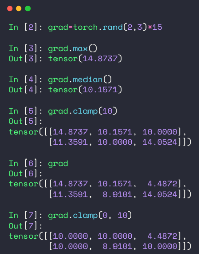
import torch

grad = torch.rand(2, 3) * 15  # 0~15随机生成
print(grad.max(), grad.min(), grad.median())  # 最大值最小值平均值

print('\ngrad =\n', grad)
print('\ngrad.norm(2) = ', grad.norm(2))
print('\ngrad.clamp(10) = \n', grad.clamp(10))  # 最小是10,小于10的都变成10
print('\ngrad.clamp(3, 10) = \n', grad.clamp(3, 10))  # 最小是3,小于3的都变成3;最大是10,大于10的都变成10

打印结果：

tensor(14.2548) tensor(3.5795) tensor(4.9580)
grad =
 tensor([[ 3.5795, 11.3405, 14.2548],
        [ 4.0516, 13.8750,  4.9580]])
grad.norm(2) =  tensor(24.0444)
grad.clamp(10) = 
 tensor([[10.0000, 11.3405, 14.2548],
        [10.0000, 13.8750, 10.0000]])
grad.clamp(3, 10) = 
 tensor([[ 3.5795, 10.0000, 10.0000],
        [ 4.0516, 10.0000,  4.9580]])

五、Tensor/张量的属性统计

1. 范数：norm()

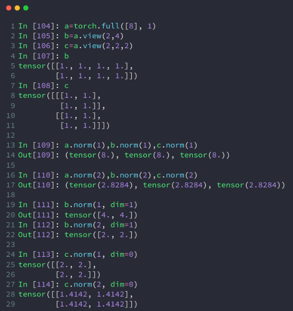
import torch

a = torch.full([8], 1)
b = a.reshape([2, 4])
c = a.reshape([2, 2, 2])

# 求L1范数(所有元素绝对值求和)
print(a.norm(1), b.norm(1), c.norm(1))
# 求L2范数(所有元素的平方和再开根号)
print(a.norm(2), b.norm(2), c.norm(2))

# 在b的1号维度上求L1范数
print(b.norm(1, dim=1))
# 在b的1号维度上求L2范数
print(b.norm(2, dim=1))

# 在c的0号维度上求L1范数
print(c.norm(1, dim=0))
# 在c的0号维度上求L2范数
print(c.norm(2, dim=0))

打印结果：

tensor(8.) tensor(8.) tensor(8.)
tensor(2.8284) tensor(2.8284) tensor(2.8284)
tensor([4., 4.])
tensor([2., 2.])
tensor([[2., 2.],
  [2., 2.]])
tensor([[1.4142, 1.4142],
  [1.4142, 1.4142]])

2、均值mean()、累加sum()、最小min()、最大max()、累积prod()

操作默认会将Tensor打平后取最大值索引和最小值索引，如果不希望Tenosr打平，而是求给定维度上的索引，需要指定在哪一个维度上求均值mean()、累加sum()、最小min()、最大max()、累积prod()。

b = torch.arange(8).reshape(2, 4).float()
print(b)
# 均值,累加,最小,最大,累积
print(b.mean(), b.sum(), b.min(), b.max(), b.prod())
# 打平后的最小最大值索引
print(b.argmax(), b.argmin())

打印结果：

tensor([[0., 1., 2., 3.],
        [4., 5., 6., 7.]])
tensor(3.5000) tensor(28.) tensor(0.) tensor(7.) tensor(0.)
tensor(7) tensor(0)

3、最小值索引argmin()、最大值索引argmax()

操作默认会将Tensor打平后取最大值索引和最小值索引，如果不希望Tenosr打平，而是求给定维度上的索引，需要指定在哪一个维度上求最大值索引或最小值索引。

import torch

b = torch.arange(8).reshape(2, 4).float()
print('b = ', b)
# 打平后的最小最大值索引
print('\nb.argmax() = {0}, b.argmin() = {1}'.format(b.argmax(), b.argmin()))

打印结果：

b =  tensor([[0., 1., 2., 3.],
        [4., 5., 6., 7.]])
b.argmax() = 7, b.argmin() = 0

注意：上面的argmax、argmin操作默认会将Tensor打平后取最大值索引和最小值索引，如果不希望Tenosr打平，而是求给定维度上的索引，需要指定在哪一个维度上求最大值索引或最小值索引。

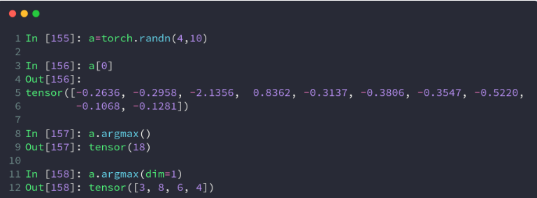
比如，有shape=[4, 10]的Tensor，表示4张图片在10分类的概率结果，我们需要知道每张图片的最可能的分类结果：

a = torch.rand(4, 10)
print(a)
# 在第二维度上求最大值索引
print(a.argmax(dim=1))

打印结果：

tensor([[0.0711, 0.5641, 0.7945, 0.6964, 0.3609, 0.5817, 0.1705, 0.6913, 0.1263,
   0.8346],
  [0.0810, 0.0771, 0.1983, 0.0344, 0.1067, 0.9591, 0.8515, 0.3046, 0.0491,
   0.1291],
  [0.3527, 0.2676, 0.9859, 0.2656, 0.1985, 0.3759, 0.8221, 0.3571, 0.5340,
   0.7759],
  [0.0969, 0.3954, 0.5478, 0.3543, 0.8253, 0.9291, 0.4960, 0.4390, 0.3780,
   0.5858]])
tensor([9, 5, 2, 5])

3、直接使用max和min配合dim参数也可以获得最值索引，同时得到最值的具体值：

print(c.max(dim=1))
1

打印结果：

(tensor([0.9589, 1.7394, 1.3448, 2.2079]), tensor([2, 2, 5, 7]))

4、使用keepdim=True

使用keepdim=True可以保持应有的dim，即仅仅是将求最值的那个dim的size变成了1，返回的结果与原Tensor维度一致。

print(c.argmax(dim=1, keepdim=True))
print(c.max(dim=1, keepdim=True))

打印结果：

tensor([[2],
  [2],
  [5],
  [7]])

(tensor([[0.9589],
  [1.7394],
  [1.3448],
  [2.2079]]), tensor([[2],
  [2],
  [5],
  [7]]))

5、取前k大/前k小/第k小的概率值及其索引：topk、kthvalue

使用topk代替max可以完成更灵活的需求，有时候不是仅仅要概率最大的那一个，而是概率最大的k个。如果不是求最大的k个，而是求最小的k个，只要使用参数largest=False，kthvalue还可以取第k小的概率值及其索引。

# 2个样本,分为10个类别的置信度
d = torch.randn(2, 10) 
# 最大概率的3个类别
print(d.topk(3, dim=1)) 
# 最小概率的3个类别
print(d.topk(3, dim=1, largest=False)) 
# 求第8小概率的类别(一共10个那就是第3大)
print(d.kthvalue(8, dim=1)) 

打印结果：

(tensor([[2.0692, 1.6490, 0.9526], [1.5983, 1.5737, 1.5532]]), tensor([[6, 3, 5], [8, 1, 2]]))
(tensor([[-1.0023, -0.6423, 0.0655], [-1.2959, -1.1504, -0.9859]]), tensor([[4, 0, 2], [0, 5, 3]]))
(tensor([0.9526, 1.5532]), tensor([5, 2]))

6、比较操作：gt、eq

import torch

a = torch.randn(2, 3)
b = torch.randn(2, 3)
print(a)
print(b)
# 比较是否大于0，是对应位置返回1，否对应位置返回0，注意得到的是ByteTensor
print(a > 0) 
print(torch.gt(a, 0))
# 是否不等于0，是对应位置返回1，否对应位置返回0
print(a != 0)
# 比较每个位置是否相等，是对应位置返回1，否对应位置返回0
print(torch.eq(a, b)) 
# 比较每个位置是否相等，全部相等时才返回True
print(torch.equal(a, b), torch.equal(a, a)) 

打印结果：

tensor([[-0.1425, -1.1142, 0.2224],
  [ 0.6142, 1.7455, -1.1776]])
tensor([[-0.0774, -1.1012, -0.4862],
  [-0.3110, -0.2110, 0.0381]])
tensor([[0, 0, 1],
  [1, 1, 0]], dtype=torch.uint8)
tensor([[0, 0, 1],
  [1, 1, 0]], dtype=torch.uint8)
tensor([[1, 1, 1],
  [1, 1, 1]], dtype=torch.uint8)
tensor([[0, 0, 0],
  [0, 0, 0]], dtype=torch.uint8)
False True

五、Tensor/张量的高阶操作

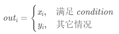
1、条件选取：torch.where(condition, x, y) → Tensor

• 返回从 x 或 y 中选择元素后形成的张量/tensor，每个元素时来自x还是来自y则取决于 condition选择器中每个元素位置的条件
  
  

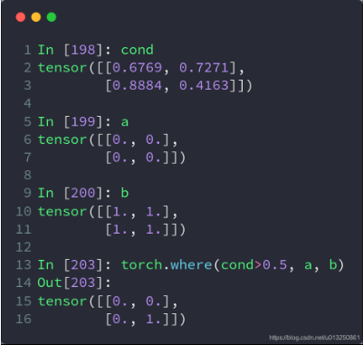
cond = torch.tensor([[0.6, 0.7], [0.3, 0.6]])
a = torch.tensor([[1., 1.], [1., 1.]])
b = torch.tensor([[0., 0.], [0., 0.]])
c = torch.where(cond > 0.5, a, b) # 此where在GPU运行，高度并行。此时cond只有0和1的值
print(c)

打印结果：

tensor([[1., 1.], [0., 1.]])

把张量中的每个数据都代入条件中，如果其大于 0 就得出 a，其它情况就得出 b，同样是把 a 和 b 的相同位置的数据导出。

2、查表搜集：torch.gather(input, dim, index, out=None) → Tensor

• 相当于查表操作

• 沿给定轴 dim，将输入索引张量 index 指定位置的值进行聚合

• 对一个3维张量，输出可以定义为：

  • out[i][j][k] = input[index[i][j][k]][j][k] # dim==0
    out[i][j][k] = input[i][index[i][j][k]][k] # dim==1
    out[i][j][k] = input[i][j][index[i][j][k]] # dim==2

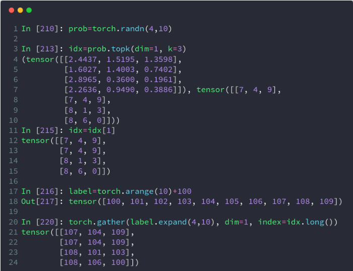
prob = torch.randn(4, 10)
idx = prob.topk(dim=1, k=3)  # prob在维度1中前三个最大的数，一共有4行，返回值和对应的下标
print("all of topk idx: ", idx)
idx = idx[1]
print("idx[1]: ", idx)
label = torch.arange(10) + 100  # 举个例子，这里的列表表示为
# 0对应于100,1对应于101，以此类推，根据实际应用修改
result = torch.gather(label.expand(4, 10), dim=1, index=idx.long())  # lable相当于one-hot编码，index表示索引
# 换而言是是y与x的函数映射关系，index表示x
print("result:", result)

打印结果：

all of topk idx:  torch.return_types.topk(
values=tensor([[0.7878, 0.2928, 0.2062],
        [0.2524, 0.2094, 0.0350],
        [1.5519, 0.8405, 0.7521],
        [1.3380, 0.9290, 0.5655]]),
indices=tensor([[2, 0, 8],
        [9, 5, 6],
        [1, 2, 0],
        [3, 7, 8]]))
idx[1]:  tensor([[2, 0, 8],
        [9, 5, 6],
        [1, 2, 0],
        [3, 7, 8]])
result: tensor([[102, 100, 108],
        [109, 105, 106],
        [101, 102, 100],
        [103, 107, 108]])

把 label 扩展为二维数据后，以 index 中的每个数据为索引，取出在 label 中索引位置的数据，再以 index 的的位置摆放。

比如，最后得出的结果中，第一行的 105 就是 label.expand(4, 10) 中第一行中索引为 5 的数据，提取出来后放在 5 所在的位置。

五、模块类

class SLNN(torch.nn.Module):
    def __init__(self, N):
        super(SLNN, self).__init__()
        self.dense1 = torch.nn.Linear(N, N)
        self.dense2 = torch.nn.Linear(N, N)
        self.tanh = torch.tanh()

    def forward(x):
        out = self.dense1(x)
        out = self.tanh(out)
        out = self.dense2(out)

六、梯度求解：

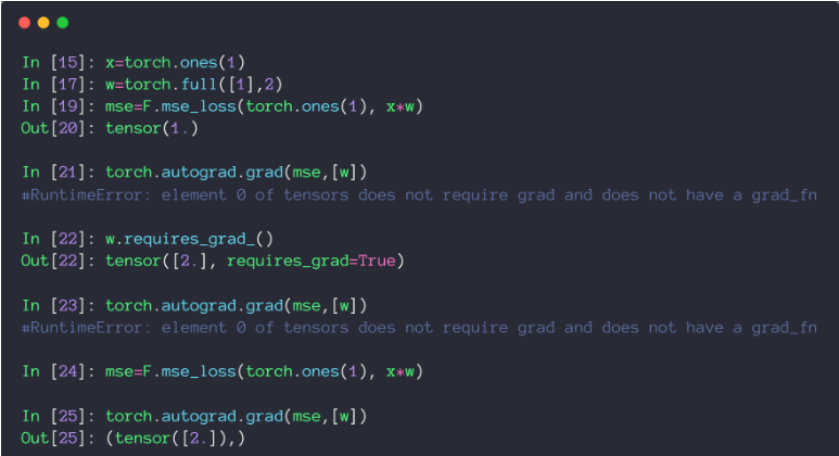
1、方法①：Autograd

• torch.autograd.grad(loss, [w1, w2,…])
  定义参数时，如果该参数需要进行求导，则需要在定义参数的时候指定其需要进行求导，否则报错。

import torch

# Autograd
# 在Tensor上的所有操作，autograd都能为它们自动提供微分
# 使得Tensor使用autograd功能，只需要设置tensor.requries_grad=True.
# Variable正式合并入Tensor, Variable本来实现的自动微分功能，Tensor就能支持
# Variable主要包含三个属性:
# data：保存Variable所包含的Tensor
# grad：保存data对应的梯度，grad也是个Variable，而不是Tensor，它和data的形状一样。
# grad_fn：指向一个Function对象，这个Function用来反向传播计算输入的梯度
x = torch.ones(2, 2, requires_grad=True)  # 为tensor设置 requires_grad 标识，代表着需要求导数
y = x.sum()
y.backward()  # 反向传播,计算梯度
print('x.grad =\n' , x.grad)  # tensor([[ 1.,  1.],[ 1.,  1.]])
x.grad.data.zero_()  # grad在反向传播过程中是累加的，每一次运行反向传播，梯度都会累加之前的梯度，所以反向传播之前需把梯度清零。
print('\nx.grad =\n' , x.grad)  # tensor([[ 0.,  0.],[ 0.,  0.]])

打印结果：

x.grad =
 tensor([[1., 1.],
        [1., 1.]])

x.grad =
 tensor([[0., 0.],
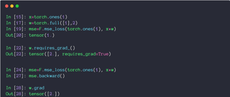
        [0., 0.]])

2、方法②：Backward()

• loss.backward()
  backward()函数用于反向求导数，使用链式法则求导，当自变量为不同变量形式时，求导方式和结果有变化。

2.1 scalar标量

import torch as t
from torch.autograd import Variable

a = Variable(t.FloatTensor([2, 3]), requires_grad=True)    # 这里为一维标量
b = a + 3
c = b * b * 3
out = c.mean()
out.backward()      
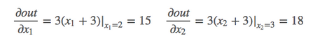
print(a.grad)       # tensor([15., 18.])

2.2 Tensor张量

# y1 = x1^2  y2 = x2^3
# dy1/dx1 | x1=2 = 2*x1 = 2*2 =4
# dy2/dx2 | x2=3 = 3*x2*x2 = 27
m = Variable(t.FloatTensor([[2, 3]]), requires_grad=True)   # 注意这里有两层括号，非标量
n = Variable(t.zeros(1, 2))
n[0, 0] = m[0, 0] ** 2
n[0, 1] = m[0, 1] ** 3

n.backward(t.Tensor([[1, 1]]),retain_graph=True)            # 这里[[1, 1]]作为梯度的系数看待
print(m.grad)              

2.3 链式求导

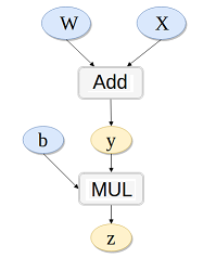
# y = x*w
# z = y + b
# k.backward(p)接受的参数p必须要和k的大小一样，x.grad = p*dk/dx
w = Variable(t.randn(3), requires_grad=True)
x = Variable(t.randn(3), requires_grad=True)
b = Variable(t.randn(3), requires_grad=True)
y = w + x
z = y.dot(b)
y.backward(b,retain_graph=True)
print(x.grad,w.grad,b)   # x.gard=w.gard=b```

# 损失函数与优化器

```python
criterion = torch.nn.MSELoss(reduction='sum')       # 定义损失函数
optimizer = torch.optim.Adam(model_eign.parameters(), lr=1e-4)      # 优化器

八、迭代

Epoch = 10000
for epoch in range(Epoch):
    y_pred = model(x)

    loss = criterion(y, y_pred)
    if epoch % 100 == 99:
        print('epoch[{}/{}],loss:{:.6f}'.format(epoch, Epoch, loss.item()))

    optimizer.zero_grad()
    loss.backward(retain_graph=True)
    optimizer.step()

九、画图

plt.plot(x.cpu(),y.cpu())           # 画图时需要临时转化变量到cpu上
plt.show()

十、合并与分割：cat、stack、Split、chunk

方法	作用	区别
cat	合并	保持原有维度的数量
stack	合并	原有维度数量加1
split	分割	按照长度去分割
chunk	分割	等分

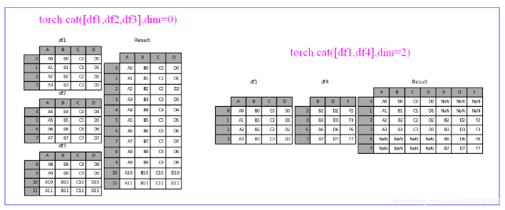
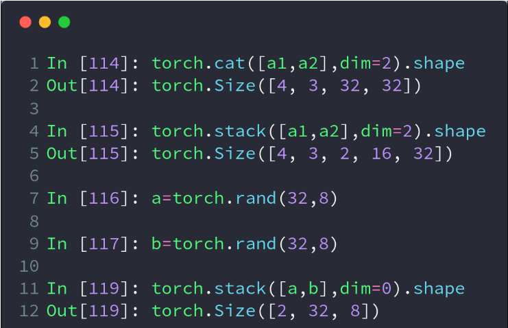
1、cat

• cat是concatenate（连接）的缩写，而不是指（猫）。作用是把2个tensor按照特定的维度连接起来。
• 要求：除被拼接的维度外，其他维度必须相同
• 源码定义：torch.cat(tensors,dim=0,out=None)
  • 第一个参数tensors是你想要连接的若干个张量，按你所传入的顺序进行连接，注意每一个张量需要形状相同，或者更准确的说，进行行连接的张量要求列数相同，进行列连接的张量要求行数相同
  • 第二个参数dim表示维度，dim=0则表示按行连接，dim=1表示按列连接
    
    

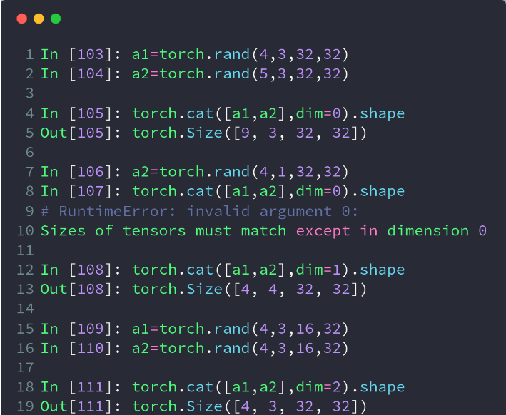
import torch
a=torch.randn(3,4) #随机生成一个shape（3，4）的tensort
b=torch.randn(2,4) #随机生成一个shape（2，4）的tensor

torch.cat([a,b],dim=0) 
#返回一个shape（5，4）的tensor
#把a和b拼接成一个shape（5，4）的tensor，
#可理解为沿着行增加的方向（即纵向）拼接

2、stack

• stack会增加一个新的维度，来表示拼接后的2个tensor，直观些理解的话，咱们不妨把一个2维的tensor理解成一张长方形的纸张，cat相当于是把两张纸缝合在一起，形成一张更大的纸，而stack相当于是把两张纸上下堆叠在一起。
• 要求：两个tensor拼接前的形状完全一致
  

a=torch.randn(3,4)
b=torch.randn(3,4)

c=torch.stack([a,b],dim=0)
#返回一个shape(2,3,4)的tensor,新增的维度2分别指向a和b

d=torch.stack([a,b],dim=1)
#返回一个shape（3,2,4）的tensor，新增的维度2分别指向相应的a的第i行和b的第i行

• 这里的关键词参数dim的理解和cat方法中有些区别。
  • cat方法中可以理解为原tensor的维度，dim=0，就是沿着原来的0轴进行拼接，dim=1，就是沿着原来的1轴进行拼接。
  • stack方法中的dim则是指向新增维度的位置，dim=0，就是在新形成的tensor的维度的第0个位置新插入维度

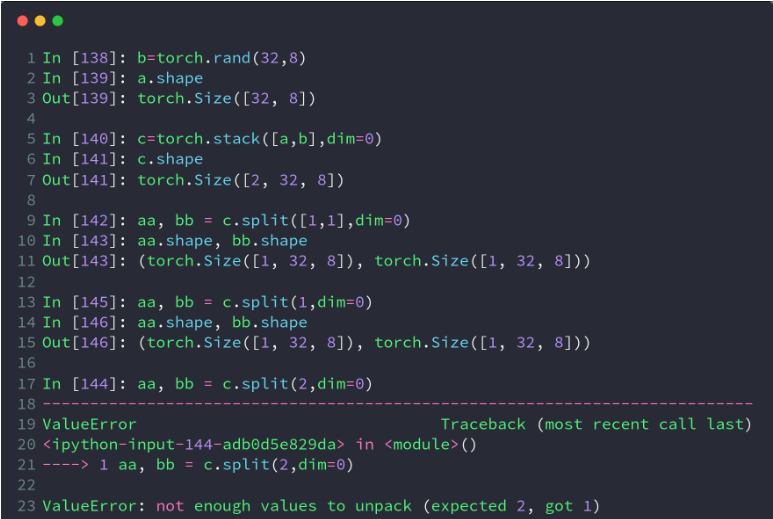
3、split

• split是根据长度去拆分tensor
• 这个函数可以说是torch.chunk（）函数的升级版本，它不仅可以按份数均匀分割，还可以按特定方案进行分割。
• 源码定义：torch.split(tensor,split_size_or_sections,dim=0)
  • 第一个参数是待分割张量
  • 第二个参数有两种形式。
  • 一种是分割份数，这就和torch.chunk()一样了。
  • 第二种这是分割方案，这是一个list，待分割张量将会分割为len（list）份，每一份的大小取决于list中的元素
  • 第三个参数为分割维度

a=torch.randn(3,4)

a.split([1,2],dim=0)
#把维度0按照长度[1,2]拆分，形成2个tensor，
#shape（1，4）和shape（2，4）

a.split([2,2],dim=1)
#把维度1按照长度[2,2]拆分，形成2个tensor，
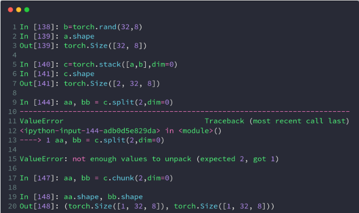
#shape（3，2）和shape（3，2）

4、chunk

• chunk可以理解为均等分的split，但是当维度长度不能被等分份数整除时，虽然不会报错，但可能结果与预期的不一样，建议只在可以被整除的情况下运用
• torch.chunk（）的作用是把一个tensor均匀分割成若干个小tensor
• 源码定义:torch.chunk(intput,chunks,dim=0)
  • 第一个参数input是你想要分割的tensor
  • 第二个参数chunks是你想均匀分割的份数，如果该tensor在你要进行分割的维度上的size不能被chunks整除，则最后一份会略小（也可能为空）
  • 第三个参数表示分割维度，dim=0按行分割，dim=1表示按列分割
  • 该函数返回由小tensor组成的list
    

a=torch.randn(4,6)

a.chunk(2,dim=0)
#返回一个shape（2，6）的tensor
a.chunk(2,dim=1)
#返回一个shape（4，3）的tensor
123456

---

---

---

参考资料：
Pytorch 常用语法
Pytorch学习笔记（一）---- 基础语法
Pytorch:Tensor的合并与分割
pytorch中torch.cat(),torch.chunk(),torch.split()函数的使用方法
Pytorch Tensor基本数学运算详解
pytorch Tensor及其基本操作
Pytorch Tensor的统计属性实例讲解
pytorch学习笔记（五）–tensor的高阶操作